Zählbezirk Wien
Zählbezirk Wien
The idea here is to get used to processing shape files (.shp) in python, by visualizing districts and counting districts (Zählbezirk) in Vienna. Vienna has 23 districts with up to 32 counting districts in each.
Dataset
In this notebook will look at use the Vienna counting district data from data.wien.gv. We’ll assume unzipped shp data is in the subdirectory OPENDATA/ZAEHLBEZIRKOGD. The data set has the following columns in addition to geometry:
AKT_TIMESTYYYY-MM-DDBEZstr 0X - (district number, 01-23)BEZNRfloat (district number 1-23)FLAECHEfloat (Area)SE_SDO_ROWint (??)UMFANGfloat (Circumference)ZBEZstr XXYY (250 unique, XX=BEZ, YY=ZBEZNR)ZBEZNRfloat (1-32)
Dependencies
We will use geopandas to do the analysis. It adds a geometry column with shapely data to a pandas dataframe to enable spatial calculations and visualization. To ebable fancy spatial joins rtree has to be installed first, get this by installing libgeospatialindex through brew install geospatialindex (or similar) and running pip install rtree. Finally run pip install geopandas.
Setup
# -- magic
%matplotlib inline
# -- imports
import os
import pandas as pd
import geopandas as gpd
from shapely.geometry import LineString
import matplotlib.pyplot as plt
# -- Globals
DATA_DIR = "OPENDATA/"  # Shape file directory is unzipped in here
FIGSIZE=(15, 10)        # Size for inline plots
# -- Helpers
# Load shape file
read_shp = lambda x: gpd.read_file(os.path.join(DATA_DIR, x))
# Create matplotlib figure and axis
fig_ax = lambda: plt.subplots(figsize=FIGSIZE)
# return variable type and value as string
vardump = lambda x: "{}: {}".format(type(x), x)
# -- GPD plot functions

def gpd_cmap(df, fig, ax, column, cmap="gray", clabel="", bbox=[0.92, 0.19, 0.03, 0.64]):
    """Plot dataframe geometry colored by by column with colorbar

    Args:
        df (GeoDataFrame): Description
        fig (figure): matplotlib figure
        ax (axis): matplotlib axis
        column (str): column in df to color by
        cmap (str, optional): colormap to use
        clabel (str, optional): label for colorbar
        bbox (list, optional): bounds for color bar
    """
    ax.set_aspect('equal')
    vmin, vmax = df[column].min(), df[column].max()
    df.plot(
        ax=ax, column=column, cmap=cmap, vmin=vmin, vmax=vmax)
    sm = plt.cm.ScalarMappable(
        cmap=cmap, norm=plt.Normalize(vmin=vmin, vmax=vmax))
    sm._A = []
    fig.colorbar(sm, label=clabel, cax=fig.add_axes(bbox))


def gpd_outline_centroid(
        df, ax, linewidth=1, linecolor="k", markersize=8, markercolor="k",
        facecolor="none", centroid=True, outline=True):
    """Plot geometry with custom fill, outline and centroid marker

    Args:
        df (GeoDataFrame): Description
        ax (TYPE): Description
        linewidth (int, optional): width of outline
        linecolor (str, optional): color of outline
        markersize (int, optional): size of centroid
        markercolor (str, optional): color of centroid
        facecolor (str, optional): color of polygon face
        centroid (bool, optional): if True draw centroid
        outline (bool, optional): if True draw outline
    """
    if outline:
        df.plot(ax=ax, linewidth=linewidth, facecolor=facecolor, color=linecolor)
    if centroid:
        df.centroid.plot(ax=ax, markersize=markersize, color=markercolor)
Prepare data
Now we load the shape file into zbzk. The columns ZBEZ and BEZNR are floats which is bad for indexing groups etc. We fix this by converting them to integers. Next we dissolve zbzk by BEZNR to get the shape of each district as bzk. Then we take the union of these to get the shape of the entire city as land. Finally we add distance dist to city center columns to zbzkand bzk, and distance bdist to bezirk center to zbzk.
# Load the shape file
zbzk = read_shp("ZAEHLBEZIRKOGD")

# Convert float bezirk number to int (helps indexing)
zbzk["ZBEZ"] = zbzk["ZBEZ"].apply(lambda x: int(x))
zbzk["BEZNR"] = zbzk["BEZNR"].apply(lambda x: int(x))

# Create frame with geometry of each bezirk
bzk = zbzk[["geometry", "BEZNR"]].dissolve(by="BEZNR")

# Create frame with total geometry
land = gpd.GeoDataFrame(geometry=[bzk.unary_union])

# Add distance to city center
cland = land.centroid[0]
zbzk["dist"] = zbzk.geometry.apply(
    lambda x: x.centroid.distance(land.centroid[0]))
bzk["dist"] = bzk.geometry.apply(
    lambda x: x.centroid.distance(land.centroid[0]))

# Add distance to bezirk center
bdists = []
for bi, b in bzk.iterrows():
    bxy = b.geometry.centroid
    bdists += [zbzk[zbzk["BEZNR"]==bi].geometry.apply(lambda x: bxy.distance(x.centroid))]
zbzk["bdist"] = pd.concat(bdists)
Plot data set overview
First we create a plotting function plt_map which plots the map to a matplot lib axis.
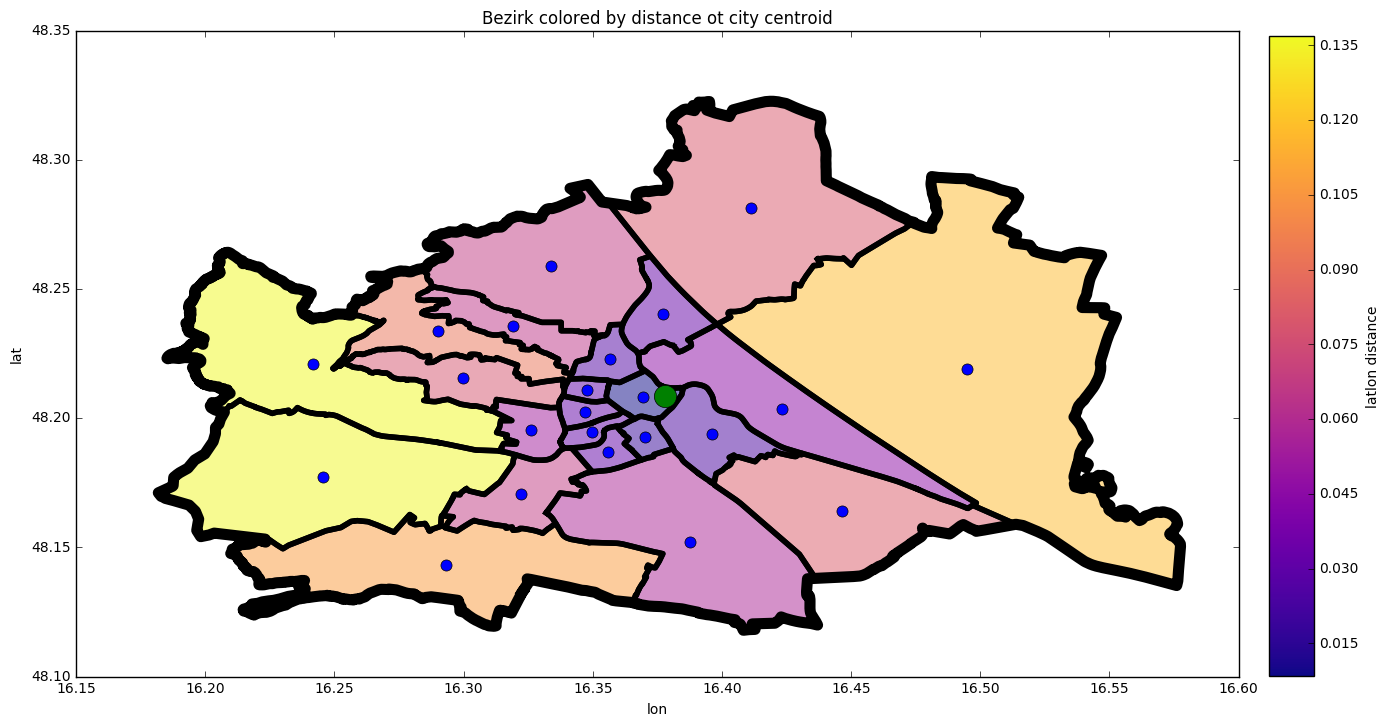
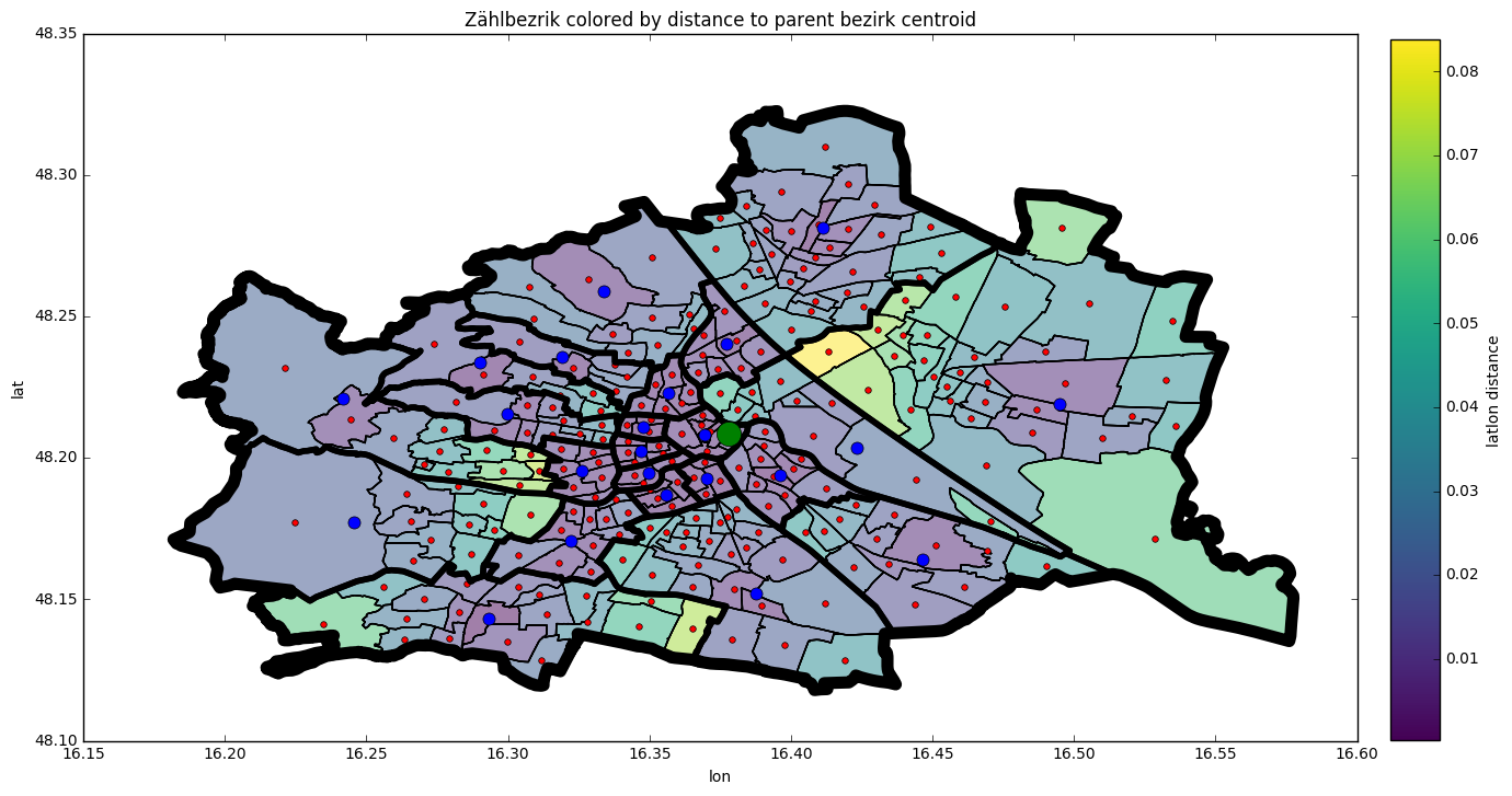
Then we use gpd_cmap to plot bzk and zbzk colored by distance to city center (dist).
def plt_map(ax, zbzk=None, bzk=None, land=None, centroid=True):
    """Plot outlines and centroids of zbzk, bzk, and land
    If any geodataframe is not given it will be skipped
    Args:
        ax (axis): matplotlib axis
        zbzk (GeoDataFrame, optional): Zählbezirk
        bzk (GeoDataFrame, optional): Bezirk
        land (GeoDataFrame, optional): Total
        centroid (bool, optional): if true draw centroid
    """
    if zbzk is not None:
        gpd_outline_centroid(
            zbzk, ax=ax, linewidth=1, centroid=centroid, markercolor="r", markersize=4)
    if bzk is not None:
        gpd_outline_centroid(
            bzk, ax=ax, linewidth=4, centroid=centroid, markercolor="b", markersize=8)
    if land is not None:
        gpd_outline_centroid(
            land, ax=ax, linewidth=8, centroid=centroid, markercolor="g", markersize=16)
    ax.set_xlabel("lon")
    ax.set_ylabel("lat")
# Do plot with latlon distance
fig, ax = fig_ax()
gpd_cmap(bzk, fig, ax, column="dist", cmap="plasma", clabel="latlon distance")
_ = ax.set_title("Bezirk colored by distance ot city centroid")
plt_map(ax, None, bzk, land)

fig, ax = fig_ax()
gpd_cmap(zbzk, fig, ax, column="bdist", cmap="viridis", clabel="latlon distance")
plt_map(ax, zbzk, bzk, land)
_ = ax.set_title("Zählbezrik colored by distance to parent bezirk centroid")


Plot smallest and largest zbrk
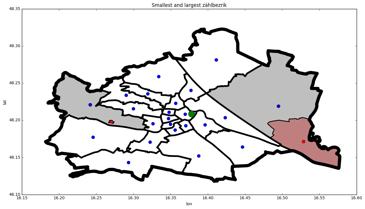
Using idxmin and idxmax the rows with extreme values can be selected. Here we use this to identify which zählbezirk has largest and smallest area (FLAECHE). We plot these red, and we plot the bezirk they belong to gray.
# Get index of min and max
fmin, fmax = zbzk["FLAECHE"].idxmin(), zbzk["FLAECHE"].idxmax()
# Extract row from zbzk at min and max
fminzbzk = zbzk.iloc[fmin: fmin + 1]
fmaxzbzk = zbzk.iloc[fmax: fmax + 1]
# Extract row from bzk with location of bezirks number
fminbzk = bzk.loc[fminzbzk["BEZNR"]]
fmaxbzk = bzk.loc[fmaxzbzk["BEZNR"]]
fig, ax = fig_ax()
ax.set_aspect('equal')
# Fill min and max bezirk in red
gpd_outline_centroid(
    fminzbzk, ax=ax, linewidth=2, markercolor="r", facecolor="red")
gpd_outline_centroid(
    fmaxzbzk, ax=ax, linewidth=2, markercolor="r", facecolor="red")
# Fill mother bezirk in gray
gpd_outline_centroid(fminbzk, ax=ax, facecolor="gray")
gpd_outline_centroid(fmaxbzk, ax=ax, facecolor="gray")
# Plot the map
plt_map(ax, None, bzk, land)
_ = plt.title("Smallest and largest zählbezrik")

Connect to center
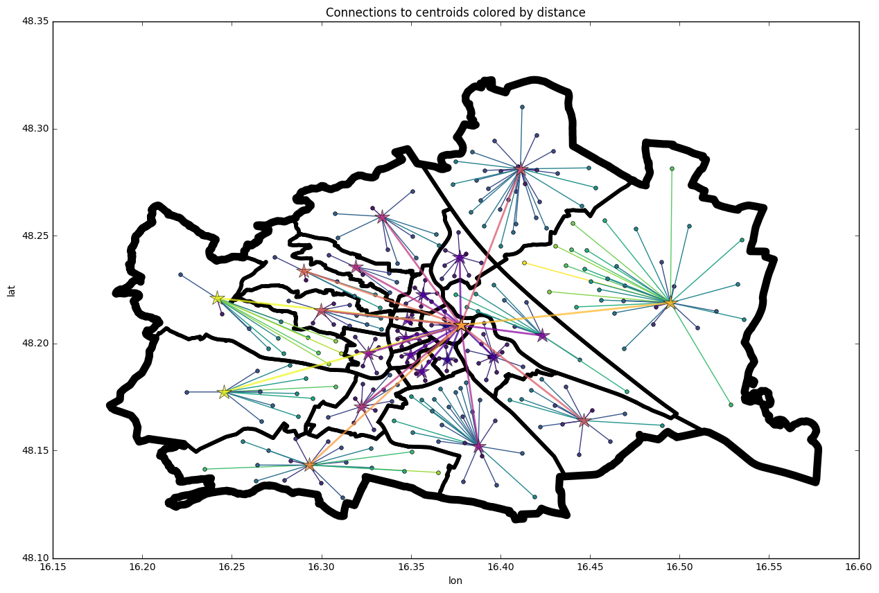
To visualize the hierarchy of the data, lets show how each zählbezirk centroid connects to its bezirk centroid, and how each bezirk connects to the total centroid.
def join_points_to_point(point, points):
    """Create [distance] and [linestring] for each joining line between point and points"""
    zdat, lines = [], []
    for p in points:
        zdat += [p.distance(point)]
        lines += [LineString([(p.x, p.y), (point.x, point.y)])]
    return zdat, lines
# Join zbzk centroids to bzk centroids
zdat, lines = [], []
for bi, b in bzk.iterrows():
    z, l = join_points_to_point(b.geometry.centroid, zbzk[zbzk["BEZNR"]==bi].centroid)
    zdat += z
    lines += l
zbzk_conn = gpd.GeoDataFrame(zdat, columns=["bdist"], geometry=lines)

# Join bzk centroids to city centroid
zdat, lines = join_points_to_point(cland, bzk.centroid)
bzk_conn = gpd.GeoDataFrame(zdat, columns=["cdist"], geometry=lines)
fig, ax = fig_ax()
plt_map(ax, None, bzk, land, centroid=False)
zbzk_conn.plot(
    ax=ax, column="bdist", marker="o", markersize=4, linewidth=1,
    cmap="viridis", zorder=2)
bzk_conn.plot(
    ax=ax, column="cdist", marker="*", markersize=16, linewidth=2,
    cmap="plasma", zorder=3, alpha=0.75)
_ = ax.set_title("Connections to centroids colored by distance")
